About a month ago I decided that I wanted to try and get a better handle on Bayesian statistical methods. I asked my advisor for some recommendations, and those included Statistical Rethinking by Richard McElreath. I got the book, but almost immediately got sidetracked. First, my wife and I went to Texas for a week to celebrate my parents’ 50th wedding anniversary. It was great to see my parents and my younger brother, and my wife and I got to do some two stepping to live country music, which is how we met and fell in love.
When we got back from Texas, I got interested in the idea of running a local LLM to help me with coding sometimes. I do a lot of my coding on a laptop and I have a separate desktop on my that I sometimes use for gaming. It has a graphics card with 12GB of memory, and there are tools that allow you to load local, open weight models into video memory for improved speed. Models that can fit into 12 GB of memory have been “quantized”, which reduces the performance and quality of LLM responses to some degree, but dramatically reduces their size. The general idea was to give myself remote access to a locally-running LLM.
I spent some time working on this and it was intermittently frustrating and interesting. I learned that if you ask a locally-running instance Qwen3.6-27B-GGUF UD-Q2_K_XL what it is, it will insist that it is an LLM hosted on the cloud. Even when you explain to it what is going on, it will continue to insist that what you are wrong and offer to help you figure out the right local model for your use-case. Perhaps one of the larger, less-quantized versions would have handled it better? I’m not sure. There were some other options I could have looked into, but I realized I wasn’t sure what goal spending a lot of time getting this working would help me accomplish. The truth is that I’m not really using Claude enough to go over the free usage tier. If I really want CLI access, I could always create an OpenRouter account. It was nice to know a local model was something I could pursue in the future if wanted to, but I was done for now.
Having updated my priors on the usefulness of running a local LLM, I decided to turn back to learning more about Bayesian methods.
Why Bayesian?
Bayesian methods have always been something interesting but kind of off into the distance. My graduate program focused primarily on frequentist methods. I knew that Bayesian models were often useful in cases where frequentist methods can break down, such as with very small samples. I had a few opportunities to dabble in it during grad school, but there was never a good project on hand that would really let me sink my teeth into it. Also, at the time everyone was using JAGS or BUGS as the software for running Bayesian models, and my experience with both of those was never especially good. Since then, STAN has come onto the scene and made running models easier (or so I hope!).
I’ve also been looking for something to give me an edge in my search, and I think Bayesian might be it. During my job search, I’ve regularly come across postings that call for experience with Bayesian inference. While I don’t know a ton about it yet, I think I’m better-positioned than a lot of data science types who come from other sorts of backgrounds. I have enough background in statistics and probability to help me get a grasp on Bayesian. I have a lot of experience with Monte Carlo simulations, which will be helpful in coming to grips with the most broadly useful method for Bayesian model estimation: Markov chain Monte Carlo (MCMC).
It would also give me something to write about, given that I had resolved to post semi-regularly on LinkedIn to keep my visibility up and help me find work.
Ok, so what is it?
You can skip this section if you know anything at all about Bayesian!
Bayesian methods take advantage of Bayes theorem, which is a method for updating your priors based on new information. That is to say, if you have an existing idea about the way the world works that you can articulate as a probability model (or a set of models), Bayes theorem will let you gather additional information and combine it with your pre-existing idea to build a new probability model. The existing idea is your prior, the additional information is your data, and the new probability model that comes of the inference machine is your posterior distribution. Assuming your priors are reasonable, the posterior distribution should be an acceptable model of what’s going on in the world. Just remember that all models are wrong, but some are useful.
Priors are useful, because researchers rarely have zero expectations or expertise about how the world functions. Harnessed correctly, researcher intuition can (I think!?) become a powerful part of the analysis process. The use of priors is also what can make Bayesian methods useful when you have limited ability to gather data. However, when you don’t have a lot of data the posterior distribution will largely reflect whatever prior you have placed on the data, so you have to be careful.
The other thing that’s nice about Bayesian is that interpretation of some of the model outputs function is more comprehensible to most people. For instance, you can use the posterior distribution to produce “credible intervals” which are essentially what most people want confidence intervals to be. A 95% credible interval for a model parameter will contain 95% of the most likely values in the posterior distribution, whereas a 95% confidence interval tells you something about the statistical precision of the parameter and not as much as you might like about the “true” value of the parameter. Instead, if a large number of researchers were to hypothetically re-run your study in the exact same way many times and they also constructed a confidence interval each time, 95% of those confidence intervals would contain the “true” value of the parameter. This is not useless, but it isn’t intuitive.
I didn’t know a lot more about Bayesian methods than this, so it was time to get reading.
I’m now a McElreath fanboy
Almost as soon as I started reading Statistical Rethinking, I was hooked. The book is written in an engaging and conversational tone, the kind of tone that has always been an ambition for my own writing. I can be impatient with introductory material in texts like this, but getting through the introduction and Chapter 1 was a breeze. Chapter 1 has a fascinating discussion of the ways that null hypothesis significance testing (NHST) fails as a form of Popperian falsification. McElreath also describes two competing theories might be represented by the same statistical model, a proposed hypothesis for a statistical test might correspond to both theories, and both theories may have the same null model. Even if you reject the null with some degree of confidence, that doesn’t help you in discriminating between competing models. Throughout the chapters I’ve read so far, McElreath’s engagement with the philosophy of science allows him to provide a really clear-eyed articulation of the value of Bayesian methods, while always keeping the limitations of all statistical inference front and center.
The book is also very funny. If you told me a Bayesian textbook was funny, I would have trouble believing you. But this textbook is funny. I have read more than one paragraph out loud to my wife (a qualitative researcher with little interest in statistics) and gotten a laugh out of her. The humor is mostly in wry asides about the world of research, so it requires a particular audience. But if you are involved in research and have a sense of humor about it, this book is funny.
In addition to his qualities as a writer, I really dig his approach to teaching this topic. All of my previous encounters with learning about Bayesian statistics involved jumping almost immediately into the use of MCMC. This approach has some merits, because many researchers want to get right into the weeds with the methods to answer their questions. I have always felt uneasy, though, because I didn’t feel like I understood what was going on “under the hood” well enough to be confident that I was doing things correctly. Statistical Rethinking doesn’t get to MCMC until Chapter 9. Instead, McElreath is invested in making you, the student, think through the nuts and bolts of simple examples to try and help you get your head around what’s really going on. He even has his own package in R that forces you to articulate every piece of the Bayesian models that most software will just tidy up for you without you having to think about it. Once you’re done with the class, you’re free (and encouraged) to use those other software packages. However, McElreath argues, when you’re learning it’s important to think hard about the boring details to make sure you really understand what’s going on. And I agree!
Many people argue that it’s silly to have to calculate a t test by hand in introductory statistics courses, because a computer will end up doing all of it for you. I have long disagreed with that argument. I have long disagreed. It is very tedious to do, but I think there’s value in grinding through the mechanics of something as simple as a t test to grant you some intuition into what’s happening inside the black box of many of the frequentist methods that researchers end up employing.
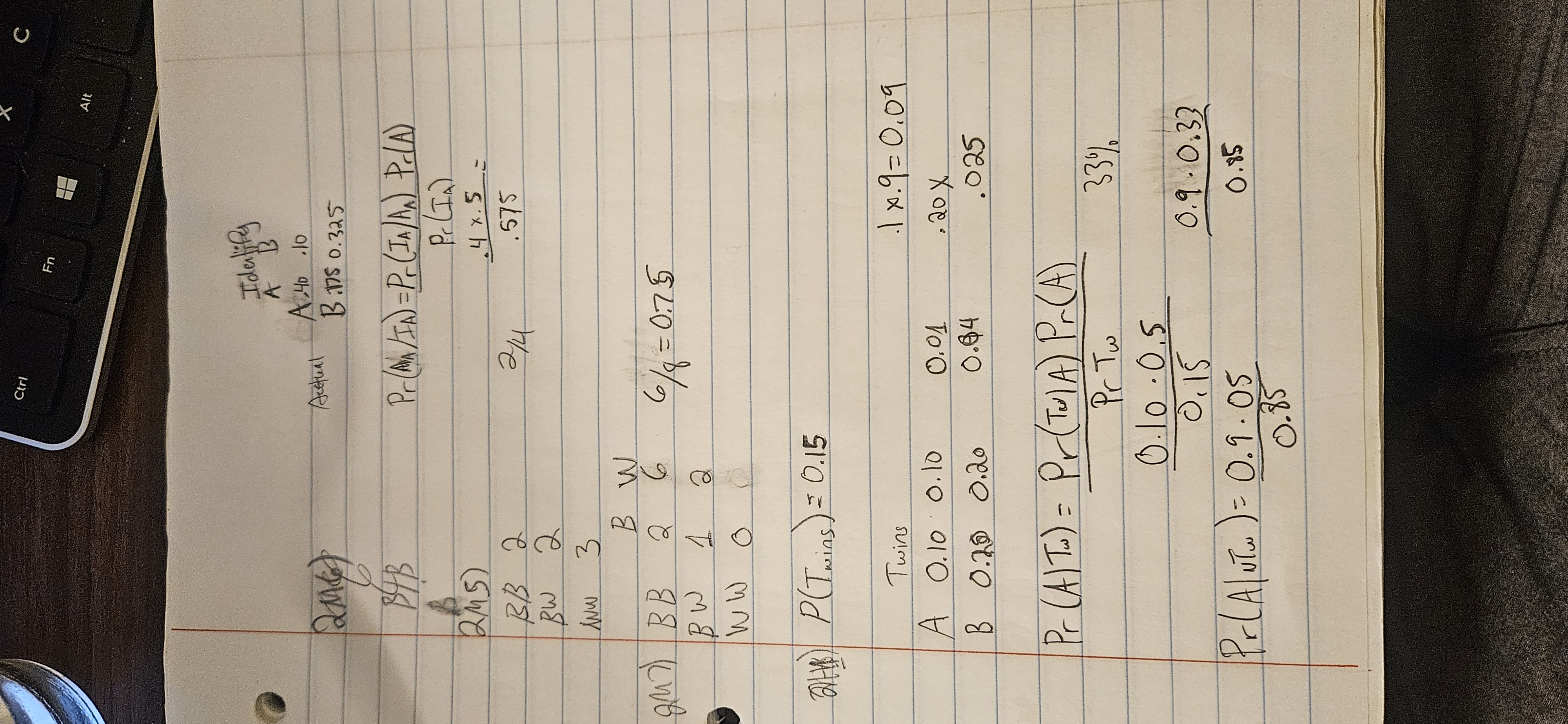
As is traditional with most textbooks, there are end-of-chapter questions testing your knowledge that are split up into easy, medium, and hard. From my perspective, even the “medium” questions are tough. I’ve got pages of scribbles that look like this:
But I’m having a lot of fun! I’m learning a lot! For instance, I’d never heard of grid approximation for estimating Bayesian models. Grid approximation is a quick-and-dirty method for estimating the posterior distribution if the posterior is simple. Rather than spinning up a complicated algorithm, you profile across a grid of equal-interval possibilities for the posterior in the parameter space. For each possible value, you multiply the probability under the prior by the likelihood for the possibility given the observed data. Each of these is now a candidate unstandardized posterior. Divide each candidate posterior by the sum of all candidate posteriors and you have a posterior probability, whichever candidate has the highest probability is now your parameter estimate. Here’s a very simple example lightly adapted from code block 2.3 in Statistical Rethinking:
This is like an instance where you have a coin with an unknown probability of coming up heads. In advance, you assume that all probabilities are equally likely. You flip it nine times, and six times it comes up heads. If you profile across 20 equally spaced values from 0 to 1, the most likely probability is 0.684. Of course, this is pretty close to a naive estimate of 6/9. That’s ok! Some exercises are just about improving your understanding.
Oher resources
In addition to the textbook, McElreath teaches Bayesian courses based around the same ideas as his text. These lectures are recorded and released on YouTube. The homework for the course along with answers are available on GitHub. All very helpful for working through this topic.